
The Nature of Charge
Perhaps one of the most fundamental yet unanswered questions in Physics is: What is (electric) charge? On WikiPedia, the following description is given:
Let us note the following:
- Charge is considered to be a property of matter;
- in this sense, it is quantized i.e. charged particles are found to exhibit a charge which is always an either positive or negative integer multiple of (an integer division of) the elementary charge, denoted by e.
Let us now introduce the (mathematical) concept of divergence:
As an intuitive explanation, one can say that the divergence describes something like the rate at which a gas, fluid or solid "thing" is expanding or contracting. When we have expansion, we have an out-going flow, while with contraction we have an inward flow.
Let us note that:
- the resulting value is calculated over an infinitesimal volume, which means something like "an infinitely small volume". This is called "taking the limit to 0", denoted by {$\lim_{\to 0}$};
- since the resulting value is divided by the volume over which the divergence is calculated, we obtain a result in the form of a density;
- since the resulting value is defined for all points in space, it essentially expresses the variation or distribution of the density value in space. That is why this notation/calculation method is called differential form;
- the differential form in vector calculus is a multi dimensional notation, wherein multiple partial differential equations are taken together in a compact notation.
For example, in normal 3 dimensional space, with vector calculus notation we don't have to write out all the partial derivatives for all 3 dimensions and combinations thereof in 3 rather long equations, but we can take them together in one vector/matrix notation, which significantly improves readability, while at the same time significantly reducing complexity and thus the chance of making errors.
This notation is specifically useful for the description of fields and it can be used to derive wave equations. The equations can also be written out and can then be numerically solved with great accuracy using a computer, which is called a simulation. This involves the implementation of the finite-difference time-domain or Yee's method (FDTD), whereby the core "bare bone" algorithm can be written down in just a few lines of computer code.
For manual mathematical analysis, however, it is often useful to use the so-called integral form of the same equations, which are essentially the same as the differential form, with the essential difference that in the integral form, we are calculating with actual volumes, surfaces, etc. without taking the limit to 0. In that case, we are not calculating with the density of a certain parameter [/m, /m2, or /m3] , but with the actual parameter. So, the differential form can always be converted to integral form, as for example with Maxwell's equations.
As an intuitive explanation, one could say that the differential form gives you a detailed view (when simulated on a computer), while the integral form gives you sort of a helicopter view of the same phenomenon.
With this in mind, it is clear that for the analytical consideration of a "toroidal topology", we would use the integral form for the calculation of parameters associated with such a topology. Such a consideration leads to rather remarkable results, as Paul Stowe has shown. Let us now review some of his work.
Stowe's aether model
The basis of Stowe's theory is the definition of a simple model for describing the aether as if it were a compressible, adiabatic and inviscid fluid. Such a fluid can be described with Euler's equations:
In other words, with such an aether model, we can describe the conservation of mass, momentum and energy and if the hypothesis of the existence of such a kind of aether holds, these are the only three quantities that are (fundamentally) conserved.
The definition of his aether model is straightforward and can be found in his "A Foundation for the Unification of Physics" (1996) (*):
With this definition, all kinds of considerations can be made, for example about the question of whether or not an aether model should be compressible or not. In a Usenet posting dated 4/26/97 he wrote(*):
{$$ div \, \mathbf{v} = 0 $$}
{$$ div \, \mathbf{v} > 0 $$}
{$$ div \, \mathbf{p} > 0 $$}
{$$ div = \lim_{V \to 0} \oint \frac{\delta A}{\delta V} \qquad \qquad \text{(A is area)}$$}
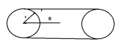
This statement illustrates the reasoning which led to Stowe's interpretation of the concept of charge, which he interprets as being a property of the field c.q. the medium. In "A Foundation for the Unification of Physics" (1996) he explained that in order to calculate the value of e, one needs to consider a torroidal topology, whereby both the enclosed volume as the surface area can be expressed in terms of the large toroidal radius, R, and the poloidal axis,r (*):
{$$ div \, S = \lim_{S \to 0} \frac{\int \delta A}{\delta S} $$}
{$$ div \, \mathbf{P} = \lim_{S \to 0} \frac{\mathbf{P} \int \delta A}{\delta S} $$}
(Image from later paper)
This is a truly remarkable finding, which finally gives us a basis for understanding what charge is and how the effect it causes, the electric field, propagates trough the medium. However, as we will see, we will have to refine Stowe's interpretation in order to come to a complete understanding of the phenomena of charge and the electric field.
Nonetheless, it is the particular idea of considering a toroidal topology within the context of the postulated existence of a physical aether which enables us to "adapt the theoretical foundation of physics to this new type of knowledge (Quantum Theory)", as Einstein once put it.
(*) Slightly edited for clarity, replaced ascii formulas with math symbols, added epmhasis, etc.
Decomposing Stowe's vector field
Now that we are aware that the consideration of a toroidal topology yields remarkable results - which can even explain some anomalies - we can apply vector calculus in order to come to a formal derivation and verification of the results acquired by Stowe, which we shall do by decomposing the field proposed by Stowe into two components. We will begin by following Stowe and define a vector field analogue to fluid dynamics, using the continuum hypothesis:
We define this vector field P as:
{$$ \mathbf{P}(\mathbf{x},t) = \rho(\mathbf{x},t) \mathbf{v}(\mathbf{x},t), $$}
where x is a point in space, $\rho(\mathbf{x},t)$ is the averaged aether density at x and $\mathbf{v}(\mathbf{x},t)$ is the local bulk flow velocity at x. Since in practice, this averaging process is usually implied, we consider the following notations to be roughly equivalent:
{$$ \mathbf{P} = \rho \mathbf{v}, $$} {$$ \mathbf{p} = m \mathbf{v}, $$} {$$ \mathbf{P} = m \mathbf{v}. $$}
We will attempt to use P for denoting the "bulk" field and p to refer to an individual "quantum", but that may not always be the case.
Helmholtz decomposition
Let us now introduce the Helmholtz decomposition:
The physical interpretation of this decomposition, is that the a given vector field can be decomposed into a longitudinal and a transverse field component:
It can be shown that performing a decomposition this way, indeed results in the Helmholtz decomposition. Also, a vector field can be uniquely specified by a prescribed divergence and curl:
{$$ \nabla \cdot \mathbf{F_v} = d \text{ and } \nabla \times \mathbf{F_v} = \mathbf{C} $$}
So, let us define a vector field {$\mathbf{A}_T$} for the magnetic potential, a scalar field {$\Phi_L$} for the electric potential, a vector field {$\mathbf{B}$} for the magnetic field, a vector field {$\mathbf{E}$} for the electric field and a vector field {$\mathbf{G}$} for the gravitational field by:
{$$ \mathbf{A}_T = \nabla \times \mathbf{v} $$} {$$ \Phi_L = \nabla \cdot \mathbf{v} $$}
{$$ \mathbf{B} = \nabla \times \mathbf{A}_T = \nabla \times (\nabla \times \mathbf{v}) $$} {$$ \mathbf{E} = - \nabla \Phi_L = - \nabla (\nabla \cdot \mathbf{v}) $$}
{$$ \mathbf{G} = \nabla \mathbf{E} = - \nabla (\nabla (\nabla \cdot \mathbf{v})) $$}
According to the above theorem, {$ \mathbf{v} $} is uniquely specified by {$\Phi_L$} and {$\mathbf{A}_T$}. And, since the Curl of the gradient of any twice-differentiable scalar field {$ \Phi $} is always the zero vector, {$\nabla \times ( \nabla \Phi ) = \mathbf{0}$}, and the divergence of the curl of any vector field P is always zero, {$\nabla \cdot ( \nabla \times \mathbf{v} ) = 0 $}, we can establish that {$\Phi_L$} is indeed curl-free and {$\mathbf{A}_T$} is indeed divergence-free.
For the summation of {$ \mathbf{E} $} and {$ \mathbf{B} $}, we get:
{$$ \mathbf{E} + \mathbf{B} = - \nabla (\nabla \cdot \mathbf{v}) + \nabla \times (\nabla \times \mathbf{v}) = - \nabla^2 \mathbf{v}, $$}
which is the negated vector Laplacian for {$ \mathbf{v} $}.
Since {$\mathbf{v}$} is uniquely specified by {$\Phi_L$} and {$\mathbf{A}_T$}, and vice versa, we can establish that with this definition, we have eliminated "gauge freedom". This clearly differentiates our definition from the usual definition of the magnetic vector potential, about which it is stated:
With our definition, we cannot add curl-free components to {$ \mathbf{v} $}, not only because {$ \mathbf{v} $} is well defined, but also because such additions would essentially be added to {$ \Phi_L $}, which encompasses the curl-free component of our decomposition.
https://en.wikipedia.org/wiki/Newton%27s_laws_of_motion#Newton.27s_second_law
{$$ \mathbf{F_N} = \frac{\mathrm{d}\mathbf{p}}{\mathrm{d}t} = \frac{\mathrm{d}(m\mathbf v)}{\mathrm{d}t} $$}
{$$ \mathbf{F_N} = m\,\frac{\mathrm{d}\mathbf{v}}{\mathrm{d}t} = m\mathbf{a}, $$}
Voor Phi kunnen we div P nemen, welke Stowe associeert met "q", maar het definieert eigenlijk de source/sinks van een flow, een flow van momenta p = m v. Dat heeft weer zo zijn gevolgen voor het beschrijven/afleiden van behoudswetten - q is immers een flow en geen "quantity" van het een of ander.
Maar goed, onder aan de WP pagina trof ik een zeeer interessante note aan:
Poloidal�toroidal decomposition for a further decomposition of the divergence-free component \nabla \times \mathbf {A}.
https://en.wikipedia.org/wiki/Poloidal%E2%80%93toroidal_decomposition
For a three-dimensional F, such that
{$$ \nabla \cdot \mathbf {F} =0, $$}
can be expressed as the sum of a toroidal and poloidal vector fields:
{$$ \mathbf {F} =\mathbf {T} +\mathbf {P} =\nabla \times \Psi \mathbf {r} +\nabla \times (\nabla \times \Phi \mathbf {r} ), $$}
where \mathbf {r} is a radial vector in spherical coordinates {\displaystyle (r,\theta ,\phi )}, and where {\mathbf {T}} is a toroidal field
{$$ \mathbf {T} =\nabla \times \Psi \mathbf {r} $$}
for scalar field {\displaystyle \Psi (r,\theta ,\phi )},[2] and where {\mathbf {P}} is a poloidal field
{$$ \mathbf {P} =\nabla \times \nabla \times \Phi \mathbf {r} $$}
for scalar field {$ \Phi (r,\theta ,\phi ) $}. This decomposition is symmetric in that the curl of a toroidal field is poloidal, and the curl of a poloidal field is toroidal"
Dit geldt dus voor een solenoidal vector veld, een divergentie-vrij vector veld:
https://en.wikipedia.org/wiki/Solenoidal_vector_field
In vector calculus a solenoidal vector field (also known as an incompressible vector field or a divergence free vector field ) is a vector field v with divergence zero at all points in the field:
{$$ \nabla \cdot \mathbf {v} =0.\, $$}
Meer over toroidal / poloidal (met een plaatje er bij): https://en.wikipedia.org/wiki/Toroidal_and_poloidal
De crux is dan dat je zowel oscillaties in de toroidale richting als in de poloidale richting kunt hebben, waarmee je een wiskundige basis hebt voor twee verschillende divergentie-vrije golf verschijnselen aka "near" en "far" fields...
Ik ga hier eens mee aan de slag....
Second derivatives
Curl of the gradient
The Curl of the gradient of any twice-differentiable scalar field {$ \phi $} is always the zero vector:
{$$\nabla \times ( \nabla \phi ) = \mathbf{0}$$}
Divergence of the curl
The divergence of the curl of any vector field A is always zero: {$$\nabla \cdot ( \nabla \times \mathbf{A} ) = 0 $$}
Divergence of the gradient
The Laplacian of a scalar field is defined as the divergence of the gradient: {$$ \nabla^2 \psi = \nabla \cdot (\nabla \psi) $$} Note that the result is a scalar quantity.
Curl of the curl
{$$ \nabla \times \left( \nabla \times \mathbf{A} \right) = \nabla(\nabla \cdot \mathbf{A}) - \nabla^{2}\mathbf{A}$$} Here,∇2 is the vector Laplacian operating on the vector field A.
Taking Gauss' law to the limit
Gauss's law may be expressed as:
{$$ \Phi_E = \frac{Q}{\varepsilon_0} $$}
where ΦE is the electric flux through a closed surface {$ S(\Omega) $} enclosing any volume {$ \Omega $}, Q is the total charge enclosed within {$ \Omega $}, and ε0 is the electric constant. The electric flux ΦE is defined as a surface integral of the electric field:
{$$ \Phi_E = \iint_{S(\Omega)} \mathbf{E} \cdot \mathrm{d}\mathbf{S} $$}
where E is the electric field, dS is a vector representing an infinitesimal element of area of the surface, and � represents the dot product of two vectors. The electric flux ΦE can also be defined as a volume integral of the charge density, which we denote by {$\rho_E$}:
{$$ \Phi_E = \frac{1}{\varepsilon_0} \iiint_\Omega \rho_E \,\mathrm{d}V $$}
Of course, the volume integral and the surface integral give the same result and thus can be equated, which is the form Gauss' law is generally included in Maxwell's equations:
{$$ \iint_{S(\Omega)} \mathbf{E}\cdot\mathrm{d}\mathbf{S} = \frac{1}{\varepsilon_0} \iiint_\Omega \rho_E \,\mathrm{d}V $$}
The above equation is written in integral form and can also be written in differential form:
{$$ div \, \mathbf{E} = \frac{\rho_E}{\varepsilon_0} \, $$}
While the integral and differential forms are mathematically equivalent by the divergence theorem, in practical application this only holds within the limitations of continuum mechanics. Also, the equations using {$\rho_E$}, the charge density, assume the charge to be uniformly distributed within the volume under consideration, which is not necessarily true under all circumstances, especially when considering a charge distribution at a very small scale, like when computing the field of a handful of particles like electrons, protons or atom nuclei at the nano-scale.
However, since within Stowe's aether model, we equate electric permittivity {$\varepsilon$} to mass density {$\rho_M$}, we can write:
{$$ \Phi_E = \iint_{S(\Omega)} \mathbf{E}\cdot\mathrm{d}\mathbf{S} = \iiint_\Omega \frac{\rho_E}{\rho_M} \,\mathrm{d}V = \frac{\rho_E}{\rho_M} |V| = \frac{Q}{M} , $$}
or:
{$$ div \, \mathbf{E} = \frac{\rho_E}{\rho_M} $$}
in the case we are considering a situation whereby there are only charge carriers within the volume under consideration.
Let us compare this with WikiPedia's definition of divergence:
{$$ div \mathbf{F}(p) = \lim_{V \rightarrow \{p\}} \iint_{S(V)} \frac{\mathbf{F} \cdot \mathbf{n}}{|V|} \; \mathrm{d}\mathbf{S} $$}
Stowe's Aether model
Now that we have formulated a basic conceptual model of electromagnetism, which requires a model of a compressible aether, we can consider how to describe such a model. Paul Stowe already proposed such a model, which he outlined as follows:
          Force     (F) -> Grad p
          Charge    (q) ->  Div p
          Magnetism (B) -> Curl p
[...]
Quantity SI Conversion Factor to Maxwell's Ether Based Units
Length meter (m) meter(m)
Mass Kilogram (kg) Kilogram (kg)
Time Second (sec) second (sec)
Force Newton (Nt) kg-m/sec^2
Energy Joules (J) kg-m^2/sec^2
Power Watts kg-m^2/sec^3
Action [h] (Planck's Const) kg-m^2/sec
Permitivitty [z] (Q^2/kg-m^3) kg/m^3 {1}
Permeability [u] (kg-m-sec^2/Q^2) m-sec^2/kg {2}
Charge [q] (Coulomb) kg/sec
Boltzmann's [k] (J/�K) m-sec
Current [I] (Amp) kg/sec^2
Electric Field [E] m/sec
Potential [V] (Voltage) m^2/sec {3}
Displacement [D] kg/m^2-sec
Resistance [R] (Ohms) m^2-sec/kg
Capacitance [C] kg/m^2
Magnetic Field [H] (Henries) m^2
Magnetic Flux [B] (Gauss) (dimensionless)
Inductance [L] m^2-sec^2/kg
Temperature [�K] (Kelvin) kg-m/sec^3
{1} - density
{2} - modulus
{3} - Kinematic Viscosity
The basic physical quantities in this system are the medium properties identified by Maxwell in his 1860-61 "On Physical Lines of Force". We quantify the mean momentum (quanta) [�], characteristic mean interaction length (quanta) [L], the root mean speed [c], and a mass attenuation coefficient [�].
Their values are,
� = 5.154664E-27 kg-m/sec L = 6.430917E-08 m � = 3.144609E-06 m^2/kg c = 2.997925E+08 m/sec
In other words, all of the major observed and measured constants of physics can be derived from the above terms.
Note that he directly associates the concept of electric elasticity with the compressibility of the aether itself, as we proposed would be necessary. He worked this out in his artlcle "The nature of Charge"(1999).
Gauss' law
Notation:
gradient : ∇
divergence: ∇⋅
curl : ∇
Note: on WP, $\rho$ is used for charge density, while in our model this is already used for mass density. In order to avoid confusion, we will use $\theta$ instead
https://en.wikipedia.org/wiki/Electric_potential#Electrostatics
{$$ V_\mathbf{E} = - \int_C \mathbf{E} \cdot \mathrm{d} \mathbf{\ell} \; , $$}
{$$ \mathbf{E} = - \mathbf{\nabla} V_\mathbf{E}. \, $$}
{$$ \mathbf{\nabla} \cdot \mathbf{E} = \mathbf{\nabla} \cdot \left (- \mathbf{\nabla} V_\mathbf{E} \right ) = -\nabla^2 V_\mathbf{E} = \theta / \varepsilon_0, \, $$}
This holds in the case the field is conservative, which means that $ \theta $ is considered to be constant over the volume wherein path C can be chosen. This also holds in infinitesimal consideration when the volume goes to zero, provided we also include the partial derivative of $ \theta $ with respect to time ($ \frac{\partial \theta}{\partial t} $).
Gauss' law in differential vorm is given as:
{$$ \mathbf{\nabla} \cdot \mathbf{E} = \frac{\theta}{\varepsilon_0} \, $$}
In Stowe's "Atomic Vortex Hypothesis", we find the following (pg. 2,3):
Thus, we can write:
{$$ \theta = \frac{\partial \rho}{\partial t} $$}
Substituting this into Gauss' equation, we get:
{$$ \mathbf{\nabla} \cdot \mathbf{E} = \frac{1}{\varepsilon_0} \frac{\partial \rho}{\partial t} $$}
This is a rather remarkable find. It fundamentally not only couples the concept of charge to the compressibility of the aether itself, it also couples it fundamentally to time variations of the mass density of the aether itself, which is quite logical given the model used for describing the aether as a super fluid, consisting of "particles" defined in terms of average momentum, or the distribution of mass times velocity.
This pretty much implies that longitudinal waves, involving the movements of aether mass, are the fundamental phenomenon that creates the electric field. This suggests that at the atomic scale, the concept of a "charge carrier" is akin to a "Helmholtz resonator" in the acoustic domain, which is capable of producing "jet streams", which can create a (propulsive) force:
http://www.youtube.com/watch?v=PoEyIJx3uM0
Notes and cut/paste stuff
http://www.tuks.nl/wiki/index.php/Main/StoweCollectedPosts
OK, let's look at "Continuum Mechanics", T. J. Chung, Prentice Hall 1988. On page 1&2 we find:
        "To distinguish the continuum or macroscopic model from a
        microscopic one, we may list a number of criteria. ... A
        concept of fundamental importance here is that of mean free
        path, which can be defined as the average distance that a
        molecule travels between successive collisions with other
        molecules.  The ratio of the mean free path L to the
        characteristic length S of the physical boundaries of interest,
        called the Knudsen number Kn, may be used to determine the
        dividing line between macroscopic and microscopic models."
Bottom line, the limit of validity of the continuum model is when L/S < 1 period. If our boxes become smaller that L we simply can't use the continuum mathematics.
http://www.tuks.nl/wiki/index.php/Main/StowePersonalEMail
The basic physical quantities in this system are the medium properties identified by Maxwell in his 1860-61 "On Physical Lines of Force". We quantify the mean momentum (quanta) [�], characteristic mean interaction length (quanta) [L], the root mean speed [c], and a mass attenuation coefficient [�].
Their values are,
� = 5.154664E-27 kg-m/sec L = 6.430917E-08 m � = 3.144609E-06 m^2/kg c = 2.997925E+08 m/sec
In other words, all of the major observed and measured constants of physics can be derived from the above terms.
https://en.wikipedia.org/wiki/Compton_wavelength
"The CODATA 2010 value for the Compton wavelength of the electron is 2.4263102389(16)�10−12 m."
So, when considering properties of the electron, we get an L/S of:
5.154664E-27 / 2.4263102389e-12 = 2.12448676899e-15,
which means we can safely use continuity mechanics at sub-atomic scales.
For Planck's length however, we get an L/S of:
https://en.wikipedia.org/wiki/Planck_length
In physics, the Planck length, denoted ℓP, is a unit of length, equal to 1.616199(97)�10−35 metres.
5.154664E-27 / 1.616199e-35 = 318937457.578
So, we certainly cannot use continuity mechanics at the Planck scale....
On uniqueness of Helmholtz decomposition:
http://www.bem.fi/book/ab/ab.htm :
 (B.14)
 (B.15)
http://arxiv.org/abs/quant-ph/0311124 :
In a Usenet posting dated 9/6/03, Stowe wrote(*):
d(rho)/dt + (rho)Div v = 0 [Eq. 1]
{$$ \frac{\partial \rho}{\partial t} + \rho \, div \, \mathbf{v} = 0 $$}
(rho)Div v = 0 [Eq. 2]
{$$ \rho \, div \, \mathbf{v} = 0 $$}
Div v = 0 [Eq. 3]
{$$ div \mathbf{v} = 0 $$}
c^2 = 1/uz [Eq. 4]
{$$ c^2 = \frac{1}{\mu z} $$}
u = 0 [Eq. 5]
{$$ \mu = 0 $$}
s(rho)Div v = s(d(rho)/dt) [Eq. 6]
{$$ s \rho \, div \, \mathbf{v} = - s \frac{\partial \rho}{\partial t}$$}
Note that Stowe made an error here. In his posting, there was no - sign, which should be there.
mDiv v = dm/dt [Eq. 7]
{$$ m div \mathbf{v} = - \frac{\partial m}{\partial t} $$}
Div v = d/dt [Eq. 8]
{$$ div \mathbf{v} = - \frac{\partial}{\partial t} $$}
As we shall see, this is the oscillation frequency of a specific "charge carrier"....
F = [1/4pi(eps)][qq/r^2] [Eq. 9]
c^2 = Y/z [Eq. 10]
c^2 = 1/u(eps) = 1/uz [Eq. 11]
E = h(nu) = 3kT [Eq. 12]
nu = q/m. [Eq. 13]
E = hq/m = 3kT [Eq. 14]
T = hq/3km [Eq. 15]
In a Usenet posting dated 5/16/97, he wrote(*):
rho = DIV D
In a Usenet posting dated 5/27/97, he wrote(*):
E = Q/4pi epsion R^2 a->
While this is a logical conclusion indeed, one must take the limitations of the used mathematics into account. In the case of Continuum Mechanics, these are well known:
[...]
In other words: when one does not take these limitations into account when using the "partial differential equations" derived this way, your equations take "on the role of master" "little by little" indeed...
Conservation laws
https://en.wikipedia.org/wiki/Fluid_dynamics#Conservation_laws
TODO
Laplace
https://en.wikipedia.org/wiki/Laplace%27s_equation
In mathematics, Laplace's equation is a second-order partial differential equation named after Pierre-Simon Laplace who first studied its properties. This is often written as:
{$$ \nabla^{2}\varphi =0 \qquad {\mbox{or}}\qquad \Delta \varphi =0 $$}
where ∆ = ∇2 is the Laplace operator and {$ \varphi $} is a scalar function.
Laplace's equation and Poisson's equation are the simplest examples of elliptic partial differential equations. The general theory of solutions to Laplace's equation is known as potential theory. The solutions of Laplace's equation are the harmonic functions, which are important in many fields of science, notably the fields of electromagnetism, astronomy, and fluid dynamics, because they can be used to accurately describe the behavior of electric, gravitational, and fluid potentials.
[...]
The Laplace equation is also a special case of the Helmholtz equation.
https://en.wikipedia.org/wiki/Vector_Laplacian
In mathematics and physics, the vector Laplace operator, denoted by {$ \nabla ^{2} $}, named after Pierre-Simon Laplace, is a differential operator defined over a vector field. The vector Laplacian is similar to the scalar Laplacian. Whereas the scalar Laplacian applies to scalar field and returns a scalar quantity, the vector Laplacian applies to the vector fields and returns a vector quantity. When computed in rectangular cartesian coordinates, the returned vector field is equal to the vector field of the scalar Laplacian applied on the individual elements.
The vector Laplacian of a vector field {$ \mathbf{A} $} is defined as
{$$ \nabla^2 \mathbf{A} = \nabla(\nabla \cdot \mathbf{A}) - \nabla \times (\nabla \times \mathbf{A}). $$}
In Cartesian coordinates, this reduces to the much simpler form:
{$$\nabla^2 \mathbf{A} = (\nabla^2 A_x, \nabla^2 A_y, \nabla^2 A_z), $$}
where {$A_x$}, {$A_y$}, and {$A_z$} are the components of {$\mathbf{A}$}. This can be seen to be a special case of Lagrange's formula; see Vector triple product.
https://en.wikipedia.org/wiki/Helmholtz_equation
In mathematics, the Helmholtz equation, named for Hermann von Helmholtz, is the partial differential equation
{$$ \nabla^2 A + k^2 A = 0 $$}
where {$ \nabla^2 $} is the Laplacian, k is the wavenumber, and A is the amplitude.
https://en.wikipedia.org/wiki/Gauss%27s_law_for_gravity
The gravitational field g (also called gravitational acceleration) is a vector field � a vector at each point of space (and time). It is defined so that the gravitational force experienced by a particle is equal to the mass of the particle multiplied by the gravitational field at that point.
Gravitational flux is a surface integral of the gravitational field over a closed surface, analogous to how magnetic flux is a surface integral of the magnetic field.
Gauss's law for gravity states:
The gravitational flux through any closed surface is proportional to the enclosed mass.
[...]
The differential form of Gauss's law for gravity states
{$$ \nabla\cdot \mathbf{g} = -4\pi G\rho, $$}
where {$\nabla\cdot$} denotes divergence, G is the universal gravitational constant, and ρ is the mass density at each point.
https://en.wikipedia.org/wiki/Divergence
It can be shown that any stationary flux v(r) that is at least twice continuously differentiable in R 3 {\displaystyle {\mathbb {R} }^{3}} {\mathbb {R} }^{3} and vanishes sufficiently fast for | r | → ∞ can be decomposed into an irrotational part E(r) and a source-free part B(r). Moreover, these parts are explicitly determined by the respective source densities (see above) and circulation densities (see the article Curl):