Introduction to the "field" concept and the modelling thereof

The above statement is a good illustration of the difference between Mathematics and Physics. In Physics, Mathematics is a fantastic tool. It allows us to make highly accurate predictions and formal descriptions of the processes we observe to take place in Nature. In a way, Mathematics is a very powerful language, because the symbols it uses and defines, have an enormous expressive power. Perhaps, above all, it is this expressive power, formalized in a language, which makes it so very useful in Physics.

It is this same expressive power, for example, which makes Python such a powerful programming language. One of the reasons Python is such an expressive programming language is because in a way "everything goes anywhere". You can add "strings" and "numbers" in Python, for example, which is a bit like adding apples and oranges in other languages. The disadvantage of such a language, however, is that sometimes errors occur when a program is being run with unexpected inputs.

The same argument can be made about Mathematics. Mathematics doesn't care if you are trying to multiply apples and oranges, even though the obtained result has no meaning in the "real world". So, what makes Mathematics such a powerful tool and language, is that because it defines all kinds of abstract concepts, relationships and calculation methods in a formal symbolic language, it has an enormous expressiveness. Expressiveness, which can be used to accurately describe all kinds of processes and systems and to solve all kinds of problems associated with these. However, it does not give a "real world" meaning to these abstract concepts it studies and describes.

So, it is not up to Mathematicians, but up to Physicists and Engineers to make sure that the Mathematics they use actually produce meaningful results. This is illustrated by Albert Einstein, who wrote in "The Evolution of Physics" (1938) (co-written with Leopold Infeld):

As we saw earlier, Freeman Dyson illustrated how Maxwell´s field model, which was founded upon well described and understood Newtonian principles, gradually evolved from a meaningful concept into a pure abstract concept, whereby eventually all connection to the "real world" has been lost:

In his paper "A Foundation for the Unification of Physics"(1996) Paul Stowe described this as follows:

Currently, the field concept has departed so much from Maxwell's down to Earth origins, that there is little room left to distinguish the modern field concept from pseudo-science, if we are to follow Karl Popper's definition:

With the current definitions of, for example, the electric-, magnetic- and gravitational fields, there are both units of measurement as well as instruments with which one can measure the strength of these fields. In hindsight, we might argue that these units of measurements are defined somewhat arbitrarily, but they are measurable nonetheless and thus "make possible the comparison with experiment".

But what about "virtual particles", "dark matter", "weak nuclear forces", "strong nuclear forces" and even "10 to 26-dimensional string theories"? Isn't there a strong sceptic argument to be made here that, at the very least, these kinds of unmeasurable concepts are bordering on the edge of pseudo-science?

Either way, even though we are well aware of the wave-particle duality principle and should have concluded that therefore there can be only One fundamental force and therefore only one field, a plethora of fields have been defined, none of which has brought us any closer to the secret of the "old one." So, if there can be only one fundamental physical field of force, what is it's Nature? How do we use this wonderful Mathematical and abstract concept of a "field" and use it in a physically meaningful way?

Let us simply go back to something that stood the test of time: the original foundation Maxwell's equations were based upon, which is to postulate the existence of a real, physical fluid-like medium wherein the same kind of flows, waves, and vortex phenomena occur as which we observe to occur in, for example, the air and waters all around us. We shall do just that and then work out the math, using nothing but "classic" Newtonian physics, meanwhile making sure that the mathematical concepts we use have a precisely defined physical meaning and produces results with well defined units of measurement.

And since it is the field concept which has made a life of it's own, let us first consider what we mean by a physical field of force and define it's units of measurement, so that we can clearly distinguish a physical field of force from the more general mathematical abstract field concept we use to describe our physical field. That way, we can do all kinds of meaningful calculations, predictions and experimental verifications. And just like 2*6=12 has no meaning in and of itself in Physics, the abstract mathematical field concept has no meaning in and of itself in Physics. To sum this up:

In a way, Physics is the art of using abstract Mathematical concepts in a way that is meaningful for describing and predicting the Physical phenomena we observe in Nature.

In practice, that comes down to a book-keeping exercise. All we really need to to is to keep track of which mathematical concept we use to describe what. For example, if we use the abstract field concept to describe something we call a physical field of force, we should unambiguously associate a unit of measurement to the abstract mathematical concept used. This way, we have clearly defined what the abstract concept means within a certain context. In Software Engineering, this is what's called type checking:

Just read "unit of measurement" for "type" and we are talking about the exact same concept.

Introduction to vector calculus

While this statement by Albert Einstein may or may not ring true to you, many people will ask the question: "What does it mean?" Since it is precisely that question that concerns us when we want to define what we mean by a "physical field of force", let us consider this statement a little bit further, because we will be using partial differential equations to describe our model, although we will make use of the expressiveness vector calculus offers us in order to keep things understandable and to express the concepts we are considering in a meaningful way.

As an illustration of the expressive power of vector calculus, let us consider the definition of "divergence":

{$$ \operatorname{div}\,\mathbf{F} = \nabla\cdot\mathbf{F} = \left( \frac{\partial}{\partial x}, \frac{\partial}{\partial y}, \frac{\partial}{\partial z} \right) \cdot (U,V,W) = \frac{\partial U}{\partial x} +\frac{\partial V}{\partial y} +\frac{\partial W}{\partial z}. $$}

At the left, we have the notation in words, followed by a notation using the $\nabla$ operator ($\nabla$ is the Greek letter "nabla"), while at the right, we have the same concept expressed in partial differential notation. So, when we use this $\nabla$ operator in equations, we are actually using partial differential equations. However, with the notation we will use, we can concentrate on the physical meaning of the equations rather than to distract and confuse ourselves with the trivial details.

So, what Einstein actually said was something like that the concepts we will use, too, gradually morphed from being useful and meaningful tools into essentially taking all branches of physics hostage. As early as 1931, Einstein already recognised that it was no longer reasoning and fundamental ideas that guided scientific progress, but rather a number of abstract concepts which drifted ever further away from having any physical meaning at all, a destructive process which still continues this very day and age.

Now let us briefly introduce the main mathematical concepts we will use: derivative, divergence, curl, gradient, the "Laplacian" and some useful vector identities. For a more in depth introduction, one can follow a free online class on multivariable calculus with exercises and instruction video's on Khan Academy.

derivatives

The vector calculus concepts we will introduced below (divergence, gradient, curl and Laplacian), are what are mathematically called derivatives:

Contrary to financial "derivatives", financial weapons of mass destruction, in mathematics a derivative of a function is, as the name suggests, a function derived from another function. It is not destructive in any way, it simply says something about a function. And what it says is not arbitrarily, but follows specific definitions. In 1 dimension, for example, the derivative of a function always gives the slope of that function, as illustrated in this WikiPedia picture:

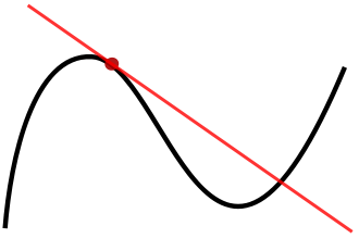
So, the mathematical concept of derivative says something about the "thing" it's the derivative of. In 1 dimension, 1D, this is always the rate of change of the function the derivative is calculated of.

Now this concept can be applied multiple times. For example, like the derivative of the position of a vehicle gives it's speed, the derivative thereof on it's turn gives you the rate of change of speed, which is called "acceleration". And since it's the second derivative of position, it's called the second derivative, or the second order derivative:

{$$ \mathbf{a} = \frac{d\mathbf{v}}{dt} = \frac{d^2\boldsymbol{x}}{dt^2}, $$}

In vector calculus, four important derivatives are defined. Three first-order ones (divergence, curl and gradient) and one second order one (Laplacian). Within this context, it is important to note the difference between a scalar and a vector (field):

• A scalar is a single number, such as for example the air pressure. And since a scalar is described a single number, it has a magnitude but does not have a direction.
• A vector contains multiple numbers and therefore has both a direction as well as a magnitude, such as for example the flow of a fluid down a hill.

Further, within vector calculus, the derivatives we use are spatial derivatives, which express the rate of change with respect to space or position rather than with respect to time:

This means that we can associate a unit of measurement to these derivatives, namely per meter [{$/m$}] for first order derivatives and per meter squared [{$/m^2$}] for second order derivatives. And since these units of measurements have a specific meaning in physics, it is most important to keep track of these throughout the whole of or model. This way, we can keep our model consistent and meaningful.

It is very important to have an intuitive interpretation of what these derivatives mean in the physical context of fluid dynamics, which is what aether physics is all about.

divergence

As an intuitive explanation, one can say that the divergence describes something like the rate at which a gas, fluid or solid "thing" is expanding or contracting. When we have expansion, we have an out-going flow, while with contraction we have an inward flow. As an analogy, consider blowing up a balloon. When you blow it up, it expands and thus we have a positive divergence. When you leave air out, it contracts and thus we have a negative divergence.

It can be both denoted as "{$ div $}" and by using the "nabla operator" as "{$ \nabla \cdot $}".

In fluid dynamics, divergence is a measurement of compression. And therefore, by definition, for an incompressible medium or vector field, the divergence is zero, like for example with the magnetic field, which is called Gauss's law for magnetism:

{$$ \nabla \cdot \mathbf{B} = 0 $$}

curl

[...]

[...]

Let us note that, unlike the divergence, the curl as both a length and a direction, which means that it gives you a vector, while the gradient gives you a single number, which is called a scalar.

gradient

The gradient concept is very similar to that of Grade or slope:

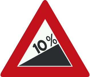
Intuitively, the gradient gives you the direction and size of the biggest change of a function. In the mountain analogy, the gradient points in the direction a ball put on a mountain surface would start rolling. The steeper the surface, the bigger the gradient.

Let us note, that unlike the divergence which takes a vector and gives you a scalar value, the gradient takes a scalar and gives you a vector. So, the gradient and the divergence are complementary to one another.

Laplacian

[...]

{$$ \Delta f = \nabla^2 f = \nabla \cdot \nabla f $$}

In this definition, the function f is a real-valued function:

This means that such a function defines a scalar field in terms of vector calculus. And therefore, it should be no surprise that the Laplacian of a scalar field {$\psi$} is defined exactly the same as the divergence of the gradient:

{$$ \nabla^2 \psi = \nabla \cdot (\nabla \psi) $$}

And since the divergence gives a scalar result, the Laplacian of a scalar field also gives a scalar result.

When we equate the Laplacian to 0, we get Laplace's equation:

{$$ \nabla^2 \phi=0, $$}

It is also used in the Wave equation {$$ \nabla^2 \psi=\frac{1}{v^2}\frac{\partial^2\psi}{\partial t^2}, $$}

the Helmholtz equation {$$ \nabla^2 \psi+k^2\psi=0, $$}

and the Schrödinger equation {$$ i\hbar \frac{\partial\Psi(x,y,z,t)}{\partial t}=\left[-\frac{\hbar^2}{2m} \nabla^2+V(x) \right] \Psi(x,y,z,t). $$}

The Laplacian can be generalized from three dimensions to four-dimensional "spacetime", which is known as the d'Alembertian or wave operator.

In the following video, the Laplacian is presented with an intuitive explanation:

http://www.youtube.com/watch?v=EW08rD-GFh0

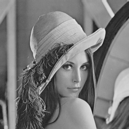
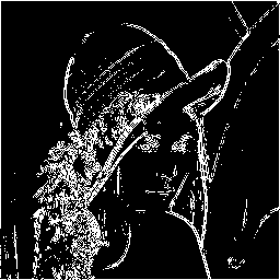
In Image Processing a Laplacian filter is used for edge detection:

Intuitive explanation

The Laplacian is analogous to the second order derivative in one dimension. At areas where the function has a (local) minimum, the Laplacian is positive, while in areas where the function has a local maximum, the Laplacian is negative. As can be seen in the above pictures, this can be used in image processing to find areas in a picture where there are large changes in brightness, which are called edges.

Vector Laplacian

The (scalar field) Laplacian concept can be generalized into vector form, the Vector Laplacian:

{$$ \nabla^2 \mathbf{A} = \nabla(\nabla \cdot \mathbf{A}) - \nabla \times (\nabla \times \mathbf{A}) $$}

From this, we can work out the curl of the curl:

{$$ \nabla \times \left( \nabla \times \mathbf{A} \right) = \nabla(\nabla \cdot \mathbf{A}) - \nabla^{2}\mathbf{A}$$}

and the gradient of the divergence:

{$$ \nabla(\nabla\cdot\mathbf{A})=\nabla^{2}\mathbf{A} + \nabla\times(\nabla\times\mathbf{A}) $$}

some vector calculus identities

Identities are equations, whereby the term left of the '=' sign gives the same result as the one on the right. So, the equations just above are examples of vector identities. We will also use the following ones:

• The curl of the gradient of any twice-differentiable scalar field {$ \phi $} is always the zero vector:

{$$\nabla \times ( \nabla \phi ) = \mathbf{0}$$}

• The divergence of the curl of any vector field A is always zero:

{$$\nabla \cdot ( \nabla \times \mathbf{A} ) = 0 $$}

Physical field of force

Now let us consider Newton's second law of motion:

{$$ \mathbf{F_N} = \frac{\mathrm{d}\mathbf{p}}{\mathrm{d}t} = \frac{\mathrm{d}(m\mathbf v)}{\mathrm{d}t} $$}

{$$ \mathbf{F_N} = m\,\frac{\mathrm{d}\mathbf{v}}{\mathrm{d}t} = m\mathbf{a}, $$}

From this, we can make an intuitive, first explanation for what a physical field of force actually is:

A physical field of force is the 3D version of the 1D concept of acceleration.

In 3D, things are more complicated, but the same principles apply. Note though, that velocity and acceleration are first and second derivatives of the position with respect to time (t).

Stowe's aether model

The basis of Stowe's theory is the definition of a simple model for describing the aether as if it were a compressible, adiabatic and inviscid fluid. Such a fluid can be described with Euler's equations:

In other words, with such an aether model, we can describe the conservation of mass, momentum and energy and if the hypothesis of the existence of such a kind of aether holds, these are the only three quantities that are (fundamentally) conserved.

The definition of his aether model is straightforward and can be found in his "A Foundation for the Unification of Physics" (1996) (*):

With this definition, all kinds of considerations can be made, for example about the question of whether or not an aether model should be compressible or not. In a Usenet posting dated 4/26/97 he wrote(*):

{$$ div \, \mathbf{v} = 0 $$}

{$$ div \, \mathbf{v} > 0 $$}

{$$ div \, \mathbf{p} > 0 $$}

{$$ div = \lim_{V \to 0} \oint \frac{\delta A}{\delta V} \qquad \qquad \text{(A is area)}$$}

This statement illustrates the reasoning which led to Stowe's interpretation of the concept of charge, which he interprets as being a property of the field c.q. the medium. In "A Foundation for the Unification of Physics" (1996) he explained that in order to calculate the value of e, one needs to consider a torroidal topology, whereby both the enclosed volume as the surface area can be expressed in terms of the large toroidal radius, R, and the poloidal axis,r (*):

(*) Slightly edited for clarity, replaced ascii formulas with math symbols, added epmhasis, etc.

high res

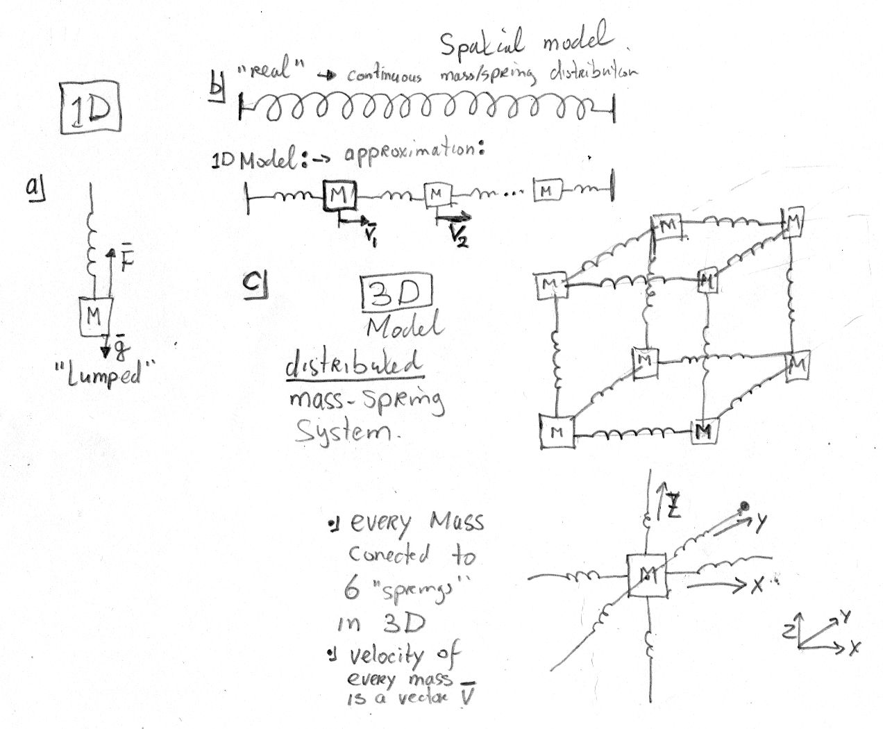
1D

1D/2D

http://www.youtube.com/watch?v=yNlOfDHyaXg

http://www.youtube.com/watch?v=xt5q3UOfG0Y

3D

Haramein's "string theory":

http://www.youtube.com/watch?v=Yb1ToYeCVnI

http://www.youtube.com/watch?v=VE520z_ugcU

Decomposing Stowe's vector field

Now that we are aware that the consideration of a toroidal topology yields remarkable results - which can even explain some anomalies - we can apply vector calculus in order to come to a formal derivation and verification of the results acquired by Stowe, which we shall do by decomposing the field proposed by Stowe into two components. We will begin by following Stowe and define a vector field analogue to fluid dynamics, using the continuum hypothesis:

We define this vector field P as:

{$$ \mathbf{P}(\mathbf{x},t) = \rho(\mathbf{x},t) \mathbf{v}(\mathbf{x},t), $$}

where x is a point in space, $\rho(\mathbf{x},t)$ is the averaged aether density at x and $\mathbf{v}(\mathbf{x},t)$ is the local bulk flow velocity at x. Since in practice, this averaging process is usually implied, we consider the following notations to be roughly equivalent:

{$$ \mathbf{P} = \rho \mathbf{v}, $$} {$$ \mathbf{p} = m \mathbf{v}, $$} {$$ \mathbf{P} = m \mathbf{v}. $$}

We will attempt to use P for denoting the "bulk" field and p to refer to an individual "quantum", but that may not always be the case.

Helmholtz decomposition

Let us now introduce the Helmholtz decomposition:

The physical interpretation of this decomposition, is that the a given vector field can be decomposed into a longitudinal and a transverse field component:

It can be shown that performing a decomposition this way, indeed results in the Helmholtz decomposition. Also, a vector field can be uniquely specified by a prescribed divergence and curl:

{$$ \nabla \cdot \mathbf{F_v} = d \text{ and } \nabla \times \mathbf{F_v} = \mathbf{C} $$}

Definition of the One field

So, let us define a vector field {$\mathbf{A}_T$} for the magnetic potential, a scalar field {$\Phi_L$} for the electric potential, a vector field {$\mathbf{B}$} for the magnetic field and a vector field {$\mathbf{E}$} for the electric field by:

{$$ \mathbf{A}_T = \nabla \times \mathbf{v} $$} {$$ \Phi_L = \nabla \cdot \mathbf{v} $$}

{$$ \mathbf{B} = \nabla \times \mathbf{A}_T = \nabla \times (\nabla \times \mathbf{v}) $$} {$$ \mathbf{E} = - \nabla \Phi_L = - \nabla (\nabla \cdot \mathbf{v}) $$}

According to the above theorem, {$ \mathbf{v} $} is uniquely specified by {$\Phi_L$} and {$\mathbf{A}_T$}. And, since the Curl of the gradient of any twice-differentiable scalar field {$ \Phi $} is always the zero vector, {$\nabla \times ( \nabla \Phi ) = \mathbf{0}$}, and the divergence of the curl of any vector field P is always zero, {$\nabla \cdot ( \nabla \times \mathbf{v} ) = 0 $}, we can establish that {$\Phi_L$} is indeed curl-free and {$\mathbf{A}_T$} is indeed divergence-free.

For the summation of {$ \mathbf{E} $} and {$ \mathbf{B} $}, we get:

{$$ \mathbf{E} + \mathbf{B} = - \nabla (\nabla \cdot \mathbf{v}) + \nabla \times (\nabla \times \mathbf{v}) = - \nabla^2 \mathbf{v}, $$}

which is the negated vector Laplacian for {$ \mathbf{v} $}.

Since {$\mathbf{v}$} is uniquely specified by {$\Phi_L$} and {$\mathbf{A}_T$}, and vice versa, we can establish that with this definition, we have eliminated "gauge freedom". This clearly differentiates our definition from the usual definition of the magnetic vector potential, about which it is stated:

With our definition, we cannot add curl-free components to {$ \mathbf{v} $}, not only because {$ \mathbf{v} $} is well defined, but also because such additions would essentially be added to {$ \Phi_L $}, which encompasses the curl-free component of our decomposition.

Notes and cut/paste stuff

While this is a logical conclusion indeed, one must take the limitations of the used mathematics into account. In the case of Continuum Mechanics, these are well known:

[...]

In other words: when one does not take these limitations into account when using the "partial differential equations" derived this way, your equations take "on the role of master" "little by little" indeed...

Conservation laws

https://en.wikipedia.org/wiki/Fluid_dynamics#Conservation_laws

TODO

Laplace

https://en.wikipedia.org/wiki/Laplace%27s_equation

In mathematics, Laplace's equation is a second-order partial differential equation named after Pierre-Simon Laplace who first studied its properties. This is often written as:

{$$ \nabla^{2}\varphi =0 \qquad {\mbox{or}}\qquad \Delta \varphi =0 $$}

where ∆ = ∇² is the Laplace operator and {$ \varphi $} is a scalar function.

Laplace's equation and Poisson's equation are the simplest examples of elliptic partial differential equations. The general theory of solutions to Laplace's equation is known as potential theory. The solutions of Laplace's equation are the harmonic functions, which are important in many fields of science, notably the fields of electromagnetism, astronomy, and fluid dynamics, because they can be used to accurately describe the behavior of electric, gravitational, and fluid potentials.

[...]

The Laplace equation is also a special case of the Helmholtz equation.

https://en.wikipedia.org/wiki/Vector_Laplacian

In mathematics and physics, the vector Laplace operator, denoted by {$ \nabla ^{2} $}, named after Pierre-Simon Laplace, is a differential operator defined over a vector field. The vector Laplacian is similar to the scalar Laplacian. Whereas the scalar Laplacian applies to scalar field and returns a scalar quantity, the vector Laplacian applies to the vector fields and returns a vector quantity. When computed in rectangular cartesian coordinates, the returned vector field is equal to the vector field of the scalar Laplacian applied on the individual elements.

The vector Laplacian of a vector field {$ \mathbf{A} $} is defined as

{$$ \nabla^2 \mathbf{A} = \nabla(\nabla \cdot \mathbf{A}) - \nabla \times (\nabla \times \mathbf{A}). $$}

In Cartesian coordinates, this reduces to the much simpler form:

{$$\nabla^2 \mathbf{A} = (\nabla^2 A_x, \nabla^2 A_y, \nabla^2 A_z), $$}

where {$A_x$}, {$A_y$}, and {$A_z$} are the components of {$\mathbf{A}$}. This can be seen to be a special case of Lagrange's formula; see Vector triple product.

https://en.wikipedia.org/wiki/Helmholtz_equation

In mathematics, the Helmholtz equation, named for Hermann von Helmholtz, is the partial differential equation

{$$ \nabla^2 A + k^2 A = 0 $$}

where {$ \nabla^2 $} is the Laplacian, k is the wavenumber, and A is the amplitude.

https://en.wikipedia.org/wiki/Gauss%27s_law_for_gravity

The gravitational field g (also called gravitational acceleration) is a vector field – a vector at each point of space (and time). It is defined so that the gravitational force experienced by a particle is equal to the mass of the particle multiplied by the gravitational field at that point.

Gravitational flux is a surface integral of the gravitational field over a closed surface, analogous to how magnetic flux is a surface integral of the magnetic field.

Gauss's law for gravity states:

The gravitational flux through any closed surface is proportional to the enclosed mass.

[...]

The differential form of Gauss's law for gravity states

{$$ \nabla\cdot \mathbf{g} = -4\pi G\rho, $$}

where {$\nabla\cdot$} denotes divergence, G is the universal gravitational constant, and ρ is the mass density at each point.

https://en.wikipedia.org/wiki/Divergence

It can be shown that any stationary flux v(r) that is at least twice continuously differentiable in R 3 {\displaystyle {\mathbb {R} }^{3}} {\mathbb {R} }^{3} and vanishes sufficiently fast for | r | → ∞ can be decomposed into an irrotational part E(r) and a source-free part B(r). Moreover, these parts are explicitly determined by the respective source densities (see above) and circulation densities (see the article Curl):