
Originally published in JBR, May-June 1986.
The Oscillating Current Transformer
The oscillating current transformer functions quite differently than a conventional transformer in that the law of dielectric inŁduction is utilized as well as the familiar law of magnetic inductŁion. The propagation of waves along the coil axis does not resemble the propagation of waves along a conventional transmission line, but is complicated by inter-turn capacitance & mutual magnetic inductance. In this respect the O.C. transformer does not behave like a resonant transmission line, nor a R.C.L. circuit, but more like a special type of wave guide. Perhaps the most important feature of the O.C. transformer is that in the course of propaŁgation along the coil axis the electric energy is dematerialized, that is, rendered mass free energy resembling Dr. Wilhelm Reich's Orgone Energy in its behavior. It is this feature that renders the O.C. transformer useful for wireless power transmission and reception, and gives the O.C. transformer singular importance in the study of Dr. Tesla's research.
FUNDAMENTALS OF COIL INDUCTION
Consider the elemental slice of a coil shown in fig. 1. Between the turns 1,2 & 3 of the coiled conductor exists a complex electric wave consisting of two basic components. In one component (fig. 2), the lines of magnetic and dielectric flux cross at right angles, producing a photon flux perpendicular to these crossings, hereby propagating energy along the gap, parallel to the conductors and around the coil. Th▒s is the transverse electro-magnetic wave. In the other component, shown in fig. 3, the lines of magnetic flux do not cross but unite along the same axis, perpendicular to the coil conductors, hereby energy is conveyed along the coil axis. This is the Longitudinal Magneto-Dielectric Wave.
Figure (1)
Figure (2)
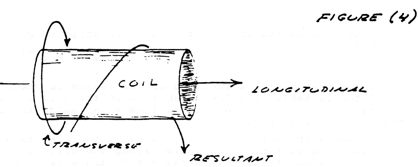
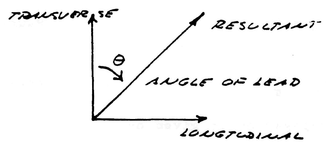
Hence, two distinct forms of energy flow are present in the coiled conductor, propagating at right angles with respect to each other, as shown in fig. 4. Hereby a resultant wave is produced which propagates around the coil in a helical fashion, leading the transverse wave between the conductors. Thus the oscillating coil posses a complex wavelength which is shorter than the waveŁlength of the coiled conductor.
COIL CALCULATION
If the assumptions are made that an alternating current is applied to one end of the coil, the other end of the coil is open circuited, Additionally external inductance and capacitance must be taken into account, then simple formulae may be derived for a single layer solenoid.
The well known formula for the total inductance of a single layer solenoid is
| $ L = \frac{r^2 N^2}{ (9r + 10l) }$ | $ x 10^{-6}$ Henry (inches) (1) |
Where:
- r is coil radius in inches
- l is coil length in inches
- N is number of turns
| $ L = \frac{31.6 r_1^2 N^2}{ (6 r_1 + 9l + 10(r_2-r_1)) }$ | microHenry |
| $ L = \frac{r^2 N^2}{ (8 r + 11w) }$ | microHenry |
Figure (3)
The capacitance of a single layer solenoid is given by the formula
| $C = pr$ | $ 2.54 x 10^{-12}$ Farads (inches) (2) |
where the factor p is a function of the length to diameter ratio, tabulated in table (1). The dimensions of the coil are shown in figure (1). The capacitance is minimum when length to diameter ratio is equal to one.
Because the coil is assumed to be in oscillation with a standŁing wave, the current distribution along the coil is not uniform, but varies sinusoidially with respect to distance along the coil. This alters the results obtained by equation (1), thus for resonance
| $L_0 = \frac12 L$ | Henrys (3) |
likewise, for capacitance
| $C_0 = \frac{8}{\pi} C$ | Farads (4) |
Hereby the velocity of propagation is given by
| $\begin{eqnarray} V_0 & = & \frac{1}{\sqrt {L_0 C_0}} \\ & = & \eta V_c \end{eqnarray}$ | Units/sec (5) |
Where
| $ V_c = \frac{1}{\sqrt {\mu \epsilon}} $ | Inch/sec (6) |
That is, the velocity of light, and
| $\begin{eqnarray} V_0 & = & \eta V_c \\ & = & \left[ \begin{array}{cc} \frac{1.77}{p} + \frac{3.94}{p}n \end{array} \right]^\frac12 \end{eqnarray}$ | $2 \pi 10^9$ Inch/sec (7) |
Where n = the ratio of coil length to coil diameter. The values of propagation factor $\eta$ are tabulated in table (2).
| $ F_{res} = (0.39 * ln(h/d) + 1.19) * 75e6 / l $ | (Hertz) |
Thus, the frequency of oscillation or resonance of the coil is given by the relation
| $ F_0 = \frac{V_0}{ (l_0 . 4) } $ | Cycles/sec (8) |
Where $l_0$ = total length of the coiled conductor in inches.
Figure (4)
The characteristic impedance of the resonant coil is given by
| $ Z_c = \sqrt {\frac{L_0}{C_0}}$ | Ohms (9) |
Hence,
| $ Z_c = N Z_s $ | Ohms (10) |
Where
| $ Z_s = \left[ \begin{array}{cc} (182.9 + 406.4n)p \end{array} \right]^\frac12 $ | $ \frac{\pi}{2} 10^3$ Ohms (inches) (11) |
and N = number of turns. The values of sheet impedance, $Z_s$, are tabulated in table (3).
The time constant of the coil, that is, the rate of energy dissipation due to coil resistance is given by the approximate formula
| $ u = \frac{R_0}{2 L_0} = ( \frac{2.72}{r}+ \frac{2.13}{l}) \pi \sqrt{F_0} $ | Nepers/sec (inches) (12) |
Where
- r = coil radius
- l = coil length
In general, the dissipation of the coil's oscillating energy by conductor resistance:
- Decreases with increase of coil diameter, d;
- Decreases with increase of coil length, l, rapidly when the ratio, n, of length to diameter is small with little decrease beyond n equal to unity;
- Is minimum when the ratio of wire diameter to coil pitch is 60%.
By examination of the attached tables, (1), (2) & (3), it is seen that the long coils of popular designs do not result in optimum performance. In general, coils should be short and wide, and not longer than n=1. The frequency is usually given as $F_0 = V_c / \lambda_0$ which by equation (7) is incorrect. Winding on solid or continuous formers rather than spaced slender rods, as shown in figure (1), greatly retards wave propagation as indicated in equation (6), thereby seriously distorting the wave. The dielectric constant of the coil,$\epsilon$ , should be as close to unity as is physically possible to insure high efficiency of transformation.
The equations for the voltampere relations of the oscillating coil are
| $ \dot E_1 = j ( Z_c Y_0 + \delta) \dot E_0 $ | Complex Input Voltage (13) |
| $ \dot I_1 = j ( Y_c Z_0 + \delta) \dot I_0 $ | Complex Input Current (14) |
| $ Z_1 = \frac{Z_c Y_0 + \delta}{Y_c Z_0 +\delta} Z_0 $ | Input Impedance, Ohms (15) |
Where
- $ \dot E_0 = $ Voltage on elevated terminal
- $ \dot I_0 = $ Current into elevated terminal
- $ Y_c = Z_c^{-1}$
- $ Z_0 = $ Terminal impedance
- $ Y_0 = $ Terminal admittance
- $ \delta = \frac{u}{2 F_0} = $ Decrement
- $ j =$ root of $\sqrt{-1}$
For negligible losses and absolute values
| $ E_1 = ( Z_c 2 \pi F_0 C_0) E_0 $ | Volts (16) |
| $ I_1 = ( Y_c / 2 \pi F_0 C_0) I_0 $ | Amperes (17) |
Where
- $C_0 =$ Terminal capacitance
By the law of conservation of energy
| $ E_1 I_1 = E_0 I_0 $ | Volt-Amperes (18) |
If the terminal capacitance is small then the approximate input/ output relations of the Tesla coil are given by
| $ E_0 = Z_c I_1 $ | Output Volts (19) |
| $ I_1 = E_0 Y_c $ | Input Amperes (20) |
| $ I_0 = Y_c E_1 $ | Output Amperes (21) |
| $ E_1 = I_0 Z_c $ | Input Volts (22) |
TABLE (1) Coil Capacitance Factor
| Length/Width = n | Factor P | Length/Width = n | Factor P |
| 0.10 | 0.96 | 0.80 | 0.46 |
| 0.15 | 0.79 | 0.90 | 0.46 |
| 0.20 | 0.70 | 1.00 | 0.46 |
| 0.25 | 0.64 | 1.5 | 0.47 |
| 0.30 | 0.60 | 2.0 | 0.50 |
| 0.35 | 0.57 | 2.5 | 0.56 |
| 0.40 | 0.54 | 3.0 | 0.61 |
| 0.45 | 0.52 | 3.5 | 0.67 |
| 0.50 | 0.50 | 4.0 | 0.72 |
| 0.60 | 0.48 | 4.5 | 0.77 |
| 0.70 | 0.47 | 5.0 | 0.81 |
TABLE (2)
| Length/Width = n | $V_0$ Inches/Sec | Percent Luminal Velocity = $\eta$ |
| 0.10 | 9.42 x 10^9 | 79.8% |
| 0.15 | 10.9 | 92.2 |
| 0.20 | 12.0 | 102 |
| 0.25 | 13.0 | 110 |
| 0.30 | 13.9 | 118 |
| 0.35 | 14.8 | 125 |
| 0.40 | 15.6 | 132 |
| 0.45 | 16.4 | 139 |
| 0.50 | 17.2 | 146 |
| 0.60 | 18.4 | 156 |
| 0.70 | 19.5 | 165 |
| 0.80 | 20.5 | 176 |
| 0.90 | 21.4 | 181 |
| 1.00 | 22.1 | 187 |
| 1.5 | 25.4 | 215 |
| 2.0 | 27.6 | 234 |
| 2.5 | 28.7 | 243 |
| 3.0 | 29.7 | 251 |
| 3.5 | 30.3 | 257 |
| 4.0 | 30.9 | 262 |
| 4.5 | 31.6 | 268 |
| 5.0 | 32.4 | 274 |
| 6.0 | 33.0 | 279 |
| 7.0 | 33.9 | 287 |
TABLE (3)
| L/W =n | $Z_s$ |
| 0.10 | 0.107 x 10 |
| 0.15 | 0.070 |
| 0.20 | 0.116 |
| 0.25 | 0.116 |
| 0.30 | 0.116 |
| 0.35 | 0.115 |
| 0.40 | 0.115 |
| 0.45 | 0.114 |
| 0.50 | 0.113 |
| 0.60 | 0.110 |
| 0.70 | 0.106 |
| 0.80 | 0.103 |
| 0.90 | 0.099 |
| 1.00 | 0.095 |
| 1.5 | 0.081 |
| 2.0 | 0.070 |
| 2.5 | 0.061 |
| 3.0 | 0.054 |
| 3.5 | 0.048 |
| 4.0 | 0.044 |
| 4.5 | 0.040 |
| 5.0 | 0.037 |
| 6.0 | 0.032 |
| 7.0 | 0.028 |
Books by Eric Dollard
CONDENSED INTRO TO TESLA TRANSFORMERS. This book is an abstract of theory and construction techniques of Tesla transformers. It is the result of experimental investigations and theoretical considerations. Includes relevant Tesla patent and an article on capacity by Fritz Lowenstein, Tesla's assistant. (BSRA #TE-1)
INTRODUCTION TO DIELECTRIC & MAGNETIC DISCHARGES IN ELECTRICAL WINDINGS, Theory of abrupt electrical oscillations such as those used by Tesla for experimental researches. Contains ELECTRICAL OSCILLAŁ TIONS IN ANTENNAE AND INDUCTION COILS by John Miller, 1919. This is one of the few articles containing equations useful to the design of Tesla coils. (BSRA #TE-2)